Understanding Homography and Inverse Perspective Mapping

First of all, congratulations. You’re finally learning something important and creating a better version of yourself! Kudos to you. Anyway, let’s get into learning IPM (Inverse Perspective Mapping)!

Why is Birds Eye View even needed? Let’s understand the importance of BEV and IPM with an example:

Imagine you’re performing lane detection. You have an epic deep learning model, let’s take UFLD (Ultra Fast Lane Detection) for now, and you perform inference on an image. Congrats! You have just received information on where the lane exists via the coordinates! LinkedIn, HERE I COME!

What can actually be done with them? You can visualize and overlay pretty lines. But you cannot drive a vehicle with them. The average pipeline is simple:

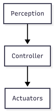
We have solved perception, but we can’t just shove these coordinates into a Stanley or Pure Pursuit controller and expect your vehicle to turn correctly. Perception tells us what exists. Controllers need geometry. Waypoints. Curvature. Lateral offset. In real-world coordinates.

What are those? Great question. You have received the lane coordinates in the image space. Pixels tend to get distorted by perspective, and they don’t have any metric meaning. IPM helps us transform those coordinates into a metric ground-plane coordinate system (I’ll talk about this later on) using linear operations.

Imagine that the lane width is 3.5 metres. In the image, at a midpoint near the ego vehicle (fancy term for our vehicle), the lanes are 400 pixels apart. A little bit further, it drops down to 300. Further away, 50 pixels. THAT is the problem that we face. As an object is going further and further away in an image, it gets smaller and smaller.

But with our new coordinates, we can establish a metric scale based on camera calibration and plane geometry, such as 1 unit in the image = 1 metre on the ground. Now that you have understood the overall use case for IPM, let’s actually understand the math behind it! Yum.

First, let’s understand what the camera actually sees

A camera maps the 3D environment to a 2D image, losing its 3rd dimension that we need (the depth). This loss is devastating in the field of perception, as now we do not know how far an object is. Of course, we can still approximately measure the distance using camera calibration and pixel size, but that is a story for another time!

Small Intro to Pinhole Cameras

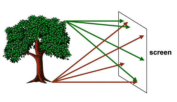
When light rays shine onto a screen, many of the rays go onto multiple points on the screen. This creates a very blurred image of the tree.

“Each point on the tree reflects light in many directions, so we’ll end up with a greenish brown smudge” — Steve Seitz

Graphics in 5 minutes — Highly recommend watching this video for pinhole perspective mapping!

But when we introduce a small hole in front of our screen and allow the light rays to shine through that hole, only specific rays get in, creating an upside-down image of the object that we want to view.

Candle image through Pinhole

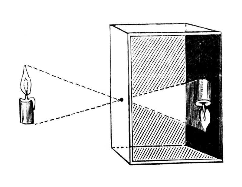
When light from the world enters the camera, it passes through a single point — the camera center (imagine the tiny hole in a pinhole camera). From there, it hits the image plane and forms a pixel. That pixel is telling you:

Something exists in this direction, but I don’t know how far it is

Now here’s the most important part:

Along the ray, there are infinitely many possible 3D points. All mapped to a single 2D pixel. It doesn’t matter if we move 1m, 10m, or 100m along the ray, all those points still map onto 1 pixel.

Can we get that 3D depth again?

No. Are we done? Not yet. We do not exactly need depth to detect lanes; we need a metric scale to judge the correct geometric shift between the pixels in the real-world coordinates. Once we know how much of a pixel shift relates to how much meters change in the real world, we can successfully move onto our control algorithms.

So if we can’t recover depth, how do we get to real-world geometry?

We cheat! Kind of. Instead of asking how far along the ray the point exists, we assume it lies on the road and ask: Where does this ray hit the ground? Basically, we want that nice metric scale to tell how many pixel coordinates cover up how much real-world coordinates.

The crucial cases we have to assume to make sure this happens are:

The ground is flat. The camera pose (fancy term for position) is fixed relative to the ground.

Because if we assume that all lane points lie on a flat ground plane, then each ray will intersect that plane at exactly one location. That intersection point is the real-world position we care about.

Now that we have assumed that the ground plane is flat, how do we translate a pixel to a metre? We will be needing a mathematical bridge between what the camera sees and what the ground actually is. To understand the transformation and the bridge, we need to hop onto a little lecture about:

Coordinate Systems and Basis Vectors!

The Default World: Standard Coordinates

Most of us are used to the standard 3D graph with x, y, and z axes. In math, these directions are defined by standard unit vectors: $\hat{i}$, $\hat{j}$, and $\hat{k}$. When we see a vector like $v = (3, 4, 2)$, it’s simply a set of driving directions: “Start at the origin (0, 0, 0). Go 3 units in the x-direction, 4 units in the y-direction, and 2 units in the z-direction.”

What is a “Basis”?

A basis is simply the underlying coordinate system — the specific set of “building blocks” you are using to measure a space. The standard x, y, and z axes are just one possible basis. You can create a completely different basis using different base vectors (like $\hat{e}_1$, $\hat{e}_2$, $\hat{e}_3$) and still represent the exact same points in space, just with different numbers. A great example would be to understand the difference between RGB (for screens) and CMY (for printers), the different color coordinate spaces.

• The RGB Basis: Think of how screens display color using Red, Green, and Blue. This is the RGB basis. To make a specific color like “CoolBlue”, the recipe might be 33 parts Red, 66 parts Green, and 99 parts Blue. So, in the RGB basis, CoolBlue = (33, 66, 99).
• The CMY Basis: Printers don’t use RGB; they use Cyan, Magenta, and Yellow (CMY). This is a totally different basis. To create the exact same CoolBlue ink on paper, the recipe changes to 222 parts Cyan, 189 parts Magenta, and 156 parts Yellow. In the CMY basis, CoolBlue = (222, 189, 156).

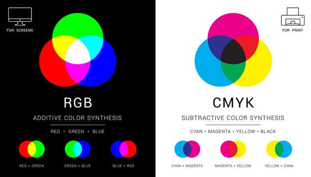
What to take away from our colorful adventure? The numbers inside the brackets do not mean anything until they have a basis (context) defined onto them. Just like printers will not respect your RGB code for a pixel because they have a different understanding of those numbers.

Colorful to Black & White

How does this basis understanding of color space relate to our image + world coordinates? Think of the road as the CMY space. The output of UFLD’s detection of the lane is in the camera basis, which gives us the pixel coordinates (480, 360) of the lane in RGB.

You can, in a sense, feed this information into a lateral (fancy term for steering) controller directly. But again, the controller expects the information (number in the brackets) in the real-world basis. If you feed camera basis coordinates into the controller, they will be misunderstood, and our vehicle will drive into a ditch, which isn’t nice.

Remember we talked about a bridge? That bridge is the Homography Matrix ($H$)!

This matrix is our ultimate translator! It takes in our input coordinates in the camera basis $(u, v)$, applies the transformation required for a change of basis, and outputs our beloved coordinate in the same physical lane location in our ground plane basis $(X, Y)$ in metres!

The Anatomy of the Translator: $H$

So, what is our bridge between the camera basis (image space) and world basis? The homography matrix ($H$) is a 3x3 grid of numbers that encapsulates all the camera’s physical properties. Its rotation, tilt, pitch, how high it is off the ground, how far it is from the middle of the ego vehicle, and its lens properties.

When we multiply our pixel coordinates by this matrix, it physically rotates, tilts, and stretches our perspective, laying those pixels flat onto the ground’s metric space. To make this happen mathematically, we perform three distinct operations: Lift, Transform and Project. We shall understand these 3 operations with code and some epic animations!

1. Lift

import numpy as np

def inverse_perspective_mapping(u, v, H):
    """
    u, v: These are the pixel coordinates from our image
    H: Our 3x3 homography matrix 
    """
    # 1st operation: LIFT 
    # Lifting the 2D coordinates into a 3D coordinate space to create a homogenous vector

    pixel_vector = np.array([[u], [v], [1]])

Lift: You can’t multiply a 3x3 matrix by a 2D coordinate $(u, v)$. The math just doesn’t fit. So, we add a 1 at the end to create a homogeneous coordinate $(u, v, 1)$. We essentially “lift” our 2D point into 3D space purely so we can do matrix math.

Visualizing the Lift operation: making our input multiplication ready.

2. Transform

    # 2nd operation: TRANSFORM
    # Matrix multiplication (The change of 'Basis')
    # H rotates and tilts the vector.
    ground_vector = H @ pixel_vector

    # This is what the raw output will look like of our matrix
    x_prime = ground_vector[0, 0]
    y_prime = ground_vector[1, 0]
    w_prime = ground_vector[2, 0]

Transform: The @ operator in Python performs the matrix multiplication. $H$ grabs our pixel vector and applies the change of basis, shifting it from the Camera world to the Ground world.

Visualizing the Transform operation: shifting the input coords into world space.

3. Project

    # 3rd operation: PROJECT
    # This is our normalization step. We divide by the third component to flatten the vector back to our 2D space

    x_ground = x_prime / w_prime
    y_ground = y_prime / w_prime

    return x_ground, y_ground

Project: The resulting vector $(x’, y’, w’)$ is still in that weird 3D homogeneous space. To push it back down into the real 2D world coordinates $(X, Y)$, we divide the first two terms by the scaling factor, $w’$.

Visualizing the Project operation: flattening the homogeneous coordinates.

Great! Now we’ll try this on an actual image!

Theory is cute, but let’s get our hands dirty. We are using the industry-standard nuScenes dataset (the v1.0-mini split) to perform Inverse Perspective Mapping on a real autonomous driving front camera. After some camera calibration magic, we get the homography matrix of the front camera:

The Real Result: From Perspective to Metric

Here is the moment of truth. On the left is the raw perspective image from the front camera. On the right is our final, warped Bird’s-Eye View:

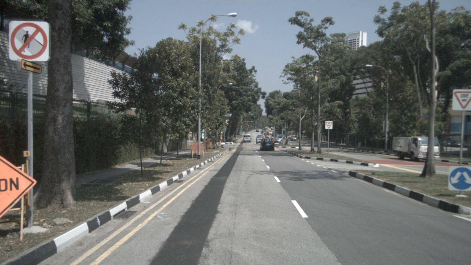
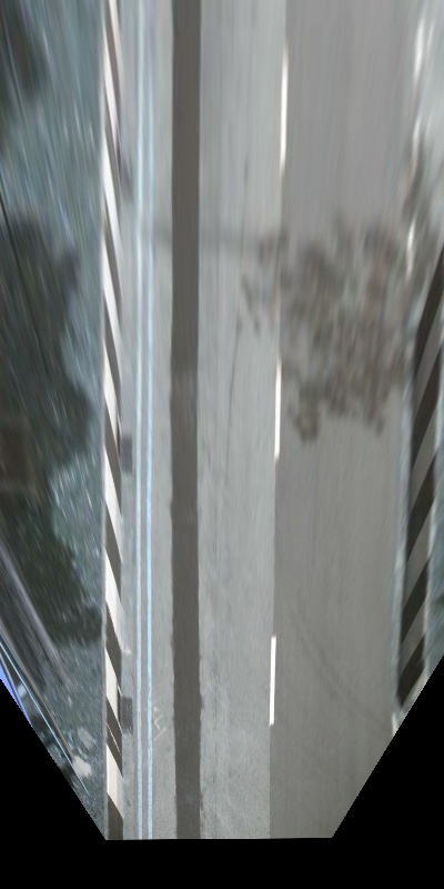
Original Image (Left) | BEV warped image (Right)

Perspective to Metric basis via IPM

This looks wild, but it is mathematically perfect IPM. Our matrix makes one huge assumption: Everything lies flat on the ground. Because the lane is flat, the lines and road texture become a perfect metric map (like a drone shot). But any 3D object sticking up from the asphalt — like the barriers or that tree — violates the assumption. The matrix “thinks” the whole tree is just pavement so it flattens it across the canvas. That smearing is the signature of a successful IPM!

Conclusion

Perception tells us what exists. Homography and IPM provide the geometry.

Let’s quickly recap what we actually accomplished here:

• The Problem: Perception models are brilliant, but they spit out useless pixel coordinates. Lateral steering controllers don’t speak “pixels” — they speak “meters”.
• The Cheat Code: By assuming the road is a perfectly flat plane, we completely bypassed the loss of depth caused by pinhole cameras.
• The Magic Bridge: We used linear algebra to build our Homography Matrix ($H$). It took our camera basis and translated it perfectly into our real-world ground basis.
• The Reality Check: We applied our Lift, Transform, Project pipeline to real nuScenes dataset imagery, proving that while 3D objects like trees might look smeared, our drivable space becomes mathematically perfect.

You’ve officially bridged the massive gap between perception and control. Keep building, keep coding, and I’ll see you on the road!

PS. All the code is available here: [My GitHub]